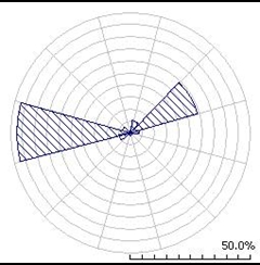
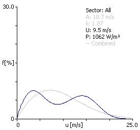
One case where the difference between these distributions is very obvious is wind climates from monsoon areas, where the wind in the monsoon and the non-monsoon seasons fall in completely different direction and magnitude ranges, as seen in the following example from India. The two dominating directional sectors (3 and 10) are seen in the wind rose (Fig. 1). The all-sector histogram of the observed (measured) wind climate (Fig. 2) is bi-modal, having a lower and a higher fraction, well separated from each other, originating mainly from sectors 3 and 10, respectively. It is clearly seen that the all-sector histogram is poorly represented by a single, fitted Weibull distribution.

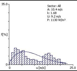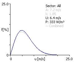
Fig. 1		Fig. 2
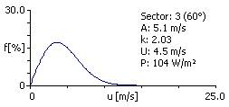
Fig. 3		Fig. 4

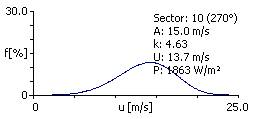
Like the observed wind climate (Fig. 2), the predicted wind climate for a wind turbine site is bi-modal as can be seen in Fig. 3 (wind distribution in sectors 3 and 10) and Fig. 4 (the all-sector distributions). The emergent distribution (solid curve) – obtained correctly as the weighted sum of the sectorial Weibull-distributions, gives a proper representation of this bi-modal character. The combined-Weibull distribution (gray curve) clearly gives a poor representation of the predicted all-sector wind speed distribution.

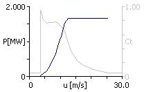
The impact on the estimation of power production, using a power curve for a 2-MW wind turbine as an example, also shows that the "Emergent" all-sector distribution is superior to use:

	Resulting AEP
	Emergent	7.679 GWh
	Combined Weibull	7.250 GWh
	Difference.............	5.59 %

In most cases, however, the the "Emergent" all-sector distributions is not bi-modal, and only a close inspection will reveal the difference from the "Combined Weibull" distribution. The case below is a typical example: