Flow Model
It is a multi-block finite-volume discretization of the in-compressible Navier-Stokes equations in general curvilinear coordinates. The code uses a co-located variable arrangement, and Rhie/Chow interpolation of Rhie (1981) to avoid odd/even pressure decoupling.
The convective terms are discretized using a third order QUICK upwind scheme, implemented using the deferred correction approach first suggested by Khosla and Rubin (1974). Central differences are used for the remaining terms.
It is parallelized with MPI for execution on distributed memory machines, using a non-overlapping domain decomposition technique and is further accelerated, using a multi-level grid sequence in steady state computations.
Model assumptions
When calculating the wind resources following the Wind Atlas method employed by WAsP, the primary concern for the CFD model is the atmospheric microscales, i.e. the near-surface wind with horizontal scales typically ranging from a few kilometres down to a few meters. The balance between large-scale pressure forces and the near-surface winds are assumed to follow the geostrophic drag law and is handled by WAsP. Coriolis forcing is therefore neglected in the CFD simulations. Also, the effect of stability is assumed to be small perturbations to the basic neutral state, and is handled by the stability model of WAsP; stability effects are therefore omitted from the CFD simulations. Due to the assumption of neutral stability and the omission of Coriolis effects, the modelled wind becomes Reynolds number independent. This means that instead of wind speed we can consider topographic speed-up ratios. The speed-up ratios calculated by the CFD model are dependent on topography only.
Reference roughness and terrain height
For any particular site of interest, the reference roughness is the “distant roughness” or the mesoscale roughness in the direction of the sector in question. For the CFD model, it is used when specifying the “boundary conditions” or farfield wind and when calculating speed-up ratios. A speed-up of, say, 5%, means that for the direction in question the actual terrain induces an increase of the wind speed of 5% as compared to a terrain with constant roughness equal to the reference roughness.
As roughnesses beyond a certain equilibrium distance have no effect on the wind at the site of interest, the reference roughness includes mainly the terrain roughnesses within that equilibrium distance (about 10 km). Roughnesses beyond the equilibrium distance are allowed only to be included with a very small weight, a weight which is decreasing with distance. Reference roughness is further described in section 8.3 of the European Wind Atlas of Troen and Petersen (1989).
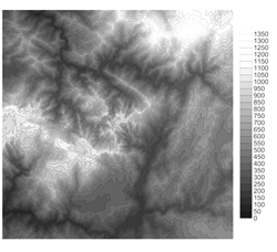
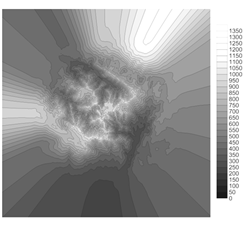
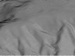
The reference terrain height is the “distance terrain height” in the direction of the sector in question. The CFD model “massages” the terrain toward this mean farfield height, as illustrated in the figure below. The CFD model effectively smoothens the far-field terrain in order to apply boundary conditions in accordance with the reference roughness.
The zooming grid of the CFD model
After having massaged the terrain the second step of the CFD process is the generation of a computational grid. The computational grid is a discretized representation of the terrain and gives the positions where the flow equations are numerically solved. Since the CFD model uses terrain-following coordinates, it is possible for the lower boundary of the computational grid to follow the topography. The CFD-model employs a high-resolution, zooming, polar grid, similar in concept to that of the IBZ model. An example of the lower boundary of the zooming grid is illustrated in the figures below. A 30 km diameter section of the Aveiro-Viseu site is shown in the upper left-hand corner of the figure. In the upper right-hand and lower left-hand closer views of the same grid are shown covering areas of 6 km by 6 km and 2 km by 2 km respectively.
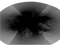
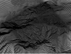
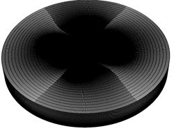
Instead of projecting the grid vertically when generating the surface grid, true surface projection is used in order to allow good resolution even in areas of very steep terrain. The grid resolution in a direction following the terrain (even e.g. vertically-aligned cliff faces) is 20 m in the 4 km by 4 km central part and gradually coarsens as you move further away. The CFD model uses a fixed domain size and grid resolution designed to model scales relevant for wind turbine siting.
To generate the 3D grid, the hyperbolic grid generator HypGrid3D (Sørensen, 1998) is used. The resolution of the grid is 5 cm near the ground and gradually coarsens with height until the top of the grid is reached at about 7000 m (depends on the terrain elevation). 96 grid points are used in the direction perpendicular to the local terrain (near-vertical direction) and about 60 % of the grid points are used in the first 300 m, giving a mean vertical resolution of about 5 m in this region. The outer boundaries of the grid are shown in the lower right-hand of the figure.
The CFD simulations
Once the CFD grid has been generated the actual CFD simulations start. In complex terrain large changes in wind speed can occur for small changes in wind direction. Because of this the CFD-model uses a 10 degree resolution and always simulates 36 wind directions.
The reference roughness for each direction is used to specify the far-field velocity and turbulence (boundary conditions) for the CFD simulations. Turbulence is modeled using the two-equation k-ε RANS model by Launder and Spalding (1974) that has been validated against other modelling approaches by Bechmann et al. (2011). Fixed model constants calibrated for atmospheric flows are used. The numerical solution of the CFD simulations is only stopped when all variable residuals have converged to under 5E-05.
Even though the CFD model calculates velocity perturbations (speed-up) and turnings at all grid points, only the results from the 2 km by 2 km central region are returned to WAsP. This is the region of highest numerical accuracy. Within this region the results are returned at fixed heights above ground (5, 10, 20, 33, 48, 65, 80, 100, 120, 150, 200, 250 and 300 m). The CFD results are therefore applicable from 5 m to 300 m above ground within the 2 km by 2 km central region.
Despite the use of proper numerical techniques, CFD results will always have a little numerical uncertainty – a form of uncertainty unknown to the IBZ-model. The right balance between computational cost and model resolution is difficult to find and must be weighed against other forms of uncertainties in the model chain. During the design of WAsP CFD the focus has been on accuracy, and a solution that leaned toward high resolution was therefore chosen. However, a few percent numerical uncertainties (1-2 %) on predicted wind speeds must be expected for sites in complex terrain.
The topography map for WAsP CFD
The below guidelines for preparing the topography map for the CFD model are much the same as for the IBZ model. However, it should be stressed that fulfilment of the guidelines is even more critical for the CFD model than for the IBZ model. In order to achieve accurate results in complex terrain, the accuracy of each and every part of the model chain needs to be very high. Since the CFD model results depend only on the terrain map (see model assumptions above), the CFD calculations should be redone if changes are made to the map. In order to achieve accurate results and avoid redoing CFD calculations, it is recommended to acquire high quality maps before running the CFD model.
Preparing the height contour map
When planning for the provision of the digital height contour map one should take the following points into consideration:
- The CFD model employs a zooming polar grid where resolution is high close to the centre of the site and gets progressively lower towards the model domain edge.
- Contrary to the IBZ model, the CFD model uses a fixed domain size (radius of 15 km) and grid resolution (grid size of 20 m) irrespectively of the digital map.
- Complex terrain affect the wind long distances downwind (“several” km)
The zooming grid of the IBZ model as well as the CFD model indicates that the contour line description close (within 2 km or so) to the prospected site(s) should be as detailed and accurate as possible (contour separation of less than 10 m), and – conversely – that the detail and accuracy may be relaxed somewhat far away from the site(s). The height contour map should preferable extend to at least 10-15 km from any (calculation) site. An adequate height contour map should therefore cover an area of at least 20 km by 20 km.
Preparing the roughness map
The roughness classification and digitisation should preferably extend to at least 15 km from any site likely to be investigated. If extensive water surfaces occur in the area, the map may even be extended to 20 km or more in the affected directions upwind from the sites of interest. An adequate roughness map should therefore cover an area of at least 30 km by 30 km.
The roughness-change line descriptions close (within 2 km or so) to the prospected site(s) should be as detailed and accurate as possible. Conversely, both the detail and accuracy may be relaxed somewhat far away from the site(s).
It is very important that the roughness map provides a coherent and consistent picture of the different roughness areas. The digitisation should be done carefully and the roughness map should be checked thoroughly using the WAsP Map Editor.
References
Bechmann, A., Sørensen, N.N., Berg, J., Mann, J. and Réthoré, P.-E. (2011). The Bolund Experiment, Part II: Blind Comparison of Microscale Flow Models. Boundary-Layer Meteorol. 141:245-271.
Khosla P. and Rubin S. (1974). A diagonally dominant second-order accurate implicit scheme. Comput Fluid 2:207—289
Launder, B. and Spalding, D. (1974). The numerical computation of turbulent flows. Comput Mech Appl Mech Eng 3:269--289
Michelsen, J.A. (1992). Basis3D – a platform for development of multiblock PDE solvers. Technical report AFM, 92-05. Technical University of Denmark, Denmark.
Michelsen, J.A. (1994). Block structured multigrid solution of 2D and 3D elliptic PPDE solvers. Technical report AFM, 94-06. Technical University of Denmark, Denmark.
Rhie, C. (1981). A numerical study of the flow past an isolated airfoil with separation. Ph.d. thesis, University of Illinois.
Sørensen, N.N. (1995). General purpose flow solver applied to flow over hill. Risø-R-827(EN). Risø National Laboratory, Roskilde, Denmark, 154 pp.
Sørensen, N.N. (1998). HypGrid2D a 2-D mesh generator. Risø-R-827(EN). Risø National Laboratory, Roskilde, Denmark.
Troen, I. And Petersen, E. (1989) European Wind Atlas. Risø National Laboratory, Roskilde. ISBN: 87-550-1482-8, 656 pp.