
Quick Guide
The figure below illustrates the process of acquiring CFD flow model results.
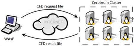
- You specify a 2 by 2 km sq. area or “tile” in WAsP. The tile coordinates and the project map is saved in a “request file”
- You uploaded the request file to Cerebrum using the “CFD Calculation Manager” tool in the WAsP Tools menu
- On Cerebrum, the CFD model will automatically start the simulations and on completion save the tile results in a “result file”
- You download the “result file” using the calculation manager and import it into WAsP.
This is the procedure for making CFD simulations in WAsP. For large wind farms you can import as many CFD tiles as necessary. Each CFD tile costs one “Calculation credit” purchased from DTU via our web-shop.
We recommend that you view the demo videos (no audio):
- How to register your license here.
- Getting the sample data set up here.
- IBZ-to-CFD walk-through here.
Step-by-step example
1. Introduction
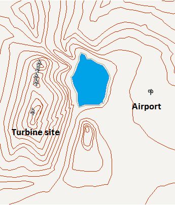
This example shows you how to predict the power yield from a wind farm using WAsP CFD. The starting point is a WAsP 10 workspace of WAsPdale. WAsPdale (see figure below) is not a complex site and the use of CFD should normally not be considered, however, most WAsP users a familiar with the site and it is therefore used in this example.
You can find information about WAsPdale in the WAsP 11 help file (“A step-by-step example”). The CFD results used in this example can be downloaded for free from here.
2. The terrain analysis
When opening the WAsPdale workspace for the first time in WAsP 11 everything looks familiar, but a closer inspection reveals changes. The figure bellow gives an example of the workspace openned in WAsP 10 (left) and in WAsP 11 (right).
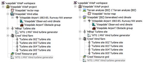
Another change is the renaming of the “Wind atlas” hierarchy member to “Generalised wind climate” and that it has been given a TA label. In this example it has an IBZ label because the IBZ model has been used to calculate the wind climate.
In order to use the CFD model in your project you need to replace the IBZ TA with a CFD TA. One way of doing this is to right-click the IBZ TA and select Convert IBZ terrain analysis to CFD. This has been done on the picture below.
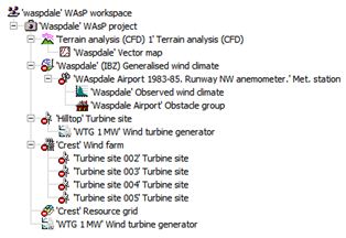
As seen, the workspace now has a 'CFD' TA and all the other hierarchy members have been marked with red "no entry" signs, meaning that you cannot do any calculation. In order to do CFD calculations you must first specify CFD tiles.
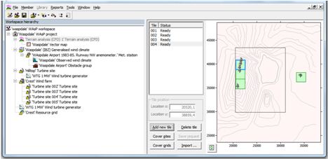
3. Specifying CFD tiles
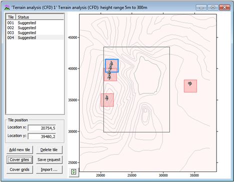
By double-clicking on the CFD TA, a new window pops up. In this window you can specify the area that you want to cover with CFD results. Since we already know the layout of the wind farm we can simply click the button Cover sites and four red “tiles” are suggested. Each tile covers a 2 by 2 sq. km area and together they cover the WAsPdale turbines sites and the met.-station. As seen, two of the tiles are overlapping – that is allowed.
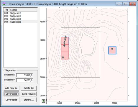
This tile-layout also covers our wind farm with CFD results, but covers a greater part of the hill crest that has wind energy potential. Since CFD computations are expensive you can justify spending a little time on the tile-layout. Once you are happy with the tile locations it is a good idea to re-click the button Cover sites. This will ensure you that all your sites are indeed covered by CFD tiles. Please note that the met.-station is also covered by a CFD tile.
Now that you have specified where you want CFD results you need to store this information in “CFD request” files, which will be sent by the Calculation Manager to the computation cluster (next section). Simply click Save request and you are asked for a file location for the four request files. Each request file contains the vector map and the position of the tile. Once the files have been saved the tile status changes from “suggested” to “pending” and the tile-colour changes from red to yellow.
4. Calculation manager
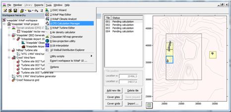
You have now saved your CFD request files and are ready to perform the CFD simulations. To do this you need to start the “WAsP CFD calculation manager” tool. This can be done by selecting it from the “Tools” menu.
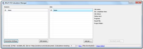
Once the job has been added the request file is uploaded to Cerebrum and the CFD simulations will start as soon as possible. A job status is given on the right side of the calculation manager.
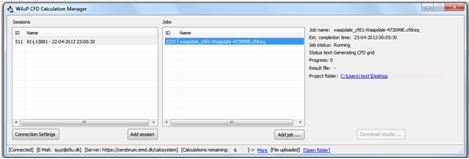
You can safely close the calculation manager tool once the job has been added. The CFD calculations are now performed automatically and Cerebrum will notify you by email when the computations are finished. When simulations are finished, you can reopen the calculation manager and click Download results ... this will save the finished CFD results to your computer. Each result file has a size of about 30 mb, so you need a reasonable fast internet connection.
5. Importing CFD results into WAsP
In the CFD TA window, back in WAsP, simply click Import ... and select the downloaded CFD results files. Once the files have been imported the tile status changes from “pending” to “ready” and the tile-colour changes from yellow to green. Also, you will notice that all the hierarchy members to the left are marked with yellow exclamation marks meaning that you are ready to do calculation
The label on Generalised wind climate is a reminder of the model used to calculate the wind climate. You should be extremely cautious about importing and using wind climates from one model together with a TA of another flow model. A wind climate calculated with an IBZ TA can be very different from one calculated by a CFD TA.
A double-click on the “Crest” Wind farm give us the calculated power productions. The power using the CFD flow model = 13.47 GWh, while the power calculated using the ‘standard WAsP’ IBZ flow model = 12.71 GWH. The CFD model therefore predicts a 6 % higher production compared to the IBZ model for this wind farm.